Linear Regression — the ML Starting Point

You already know this algorithm

If you've ever added a trendline to a scatter plot in Excel, you've done linear regression. You had data points, you drew a line through them, and you used that line to estimate values between or beyond your measurements.

That's it. That's linear regression. ML doesn't change the fundamental idea — it just gives it a proper mathematical foundation, makes it work with dozens of variables instead of two, and provides tools to measure how good the fit actually is.

Linear regression is the simplest ML algorithm, which is exactly why we're starting here. Not because it's a toy — it's used in production every day across engineering — but because every concept you learn with linear regression (how the model learns, how it measures error, how it improves) carries forward to every other algorithm. Understand this one well, and the rest will feel like variations on a theme.

How linear regression works

The idea is beautifully simple: find the line (or plane, or hyperplane) that best fits the data.

With one input variable, that's a line:

With two input variables, it's a flat plane through 3D space. With 15 input variables, it's a hyperplane in 16-dimensional space — impossible to visualise but mathematically identical.

Each input variable gets its own weight (also called a coefficient). The weight tells you how much that input affects the output. A large positive weight means "when this input goes up, the output goes up a lot." A weight near zero means "this input barely matters."

For example, suppose you're predicting surface roughness from three CNC parameters:

The weights tell you a story: feed rate has the strongest influence (0.8), depth of cut matters moderately (0.3), and spindle speed has a small negative effect (−0.1). The intercept (1.2) is the baseline roughness when all inputs are zero — often not physically meaningful, but mathematically necessary.

This is already useful engineering insight, before you even make a prediction. Linear regression doesn't just predict — it tells you which inputs matter and how much. That interpretability is one of the reasons it remains popular despite being the simplest algorithm in the toolbox.

But how does the model find the right weights?

This is where ML goes beyond what you do manually in Excel. When you click "add trendline," the software finds the best line automatically. But what does "best" actually mean? And how does it find it?

The answer leads us to one of the most fundamental concepts in all of machine learning: the cost function.

The cost function: how the model knows it's wrong

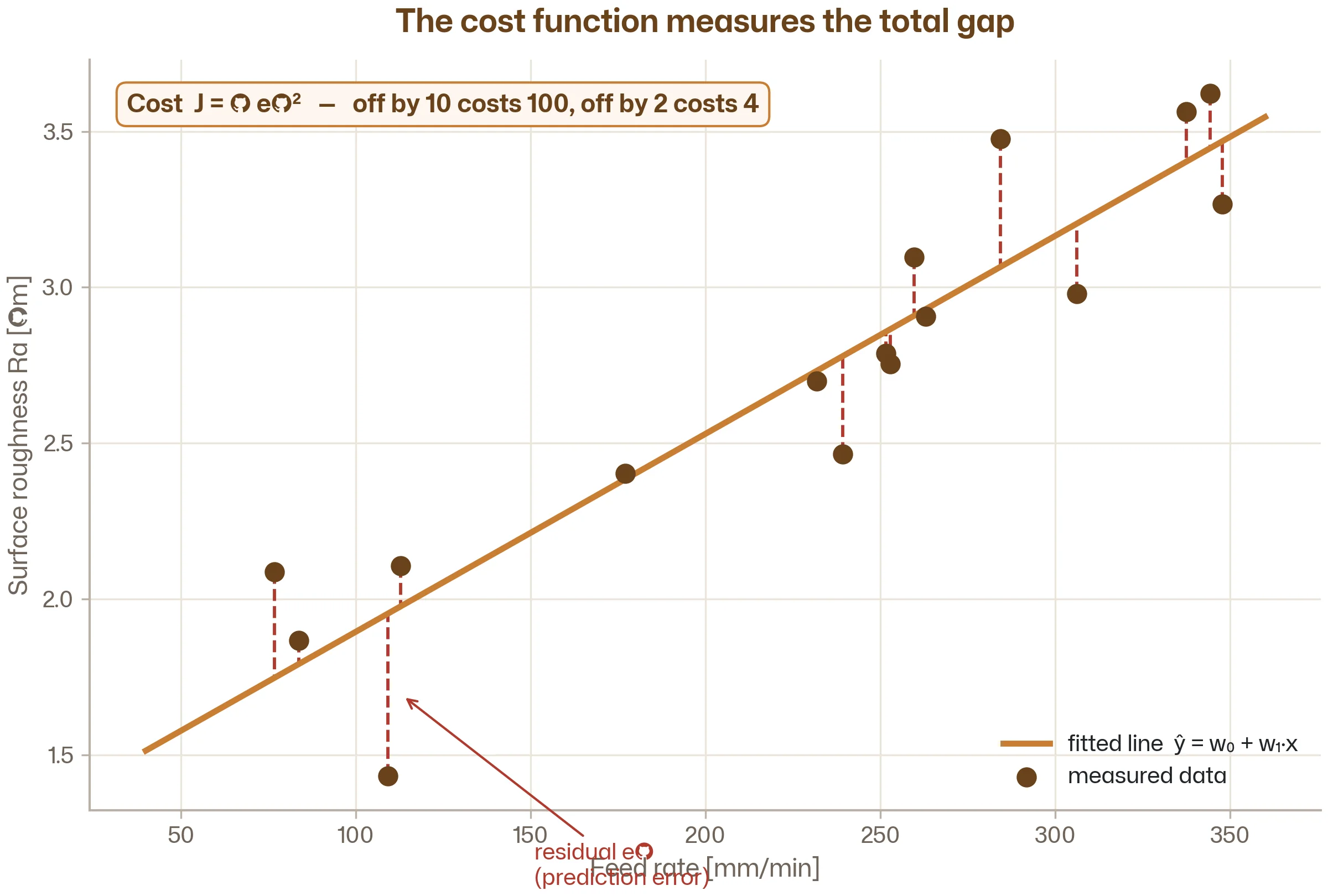
A cost function (also called a loss function) is simply a number that measures how wrong the model's predictions are. The smaller the cost, the better the model fits the data.

For linear regression, the most common cost function is the mean squared error (MSE): take each prediction, subtract the actual value, square the difference, and average across all data points.

Why squared? Two reasons. First, it treats over-predictions and under-predictions equally (squaring makes everything positive). Second, it penalises large errors much more than small ones — a prediction that's off by 10 contributes 100 to the cost, while one that's off by 2 contributes only 4. In engineering terms, this is similar to how you might use RMS error rather than mean absolute error when evaluating a measurement system.

The cost function is the model's quality metric. Every ML algorithm — not just linear regression — has one. It's the answer to "how does the model know if it's improving?" It measures the prediction error, calculates a number, and tries to make that number smaller.

Finding the best weights: two approaches

Once you have a cost function, training the model becomes an optimisation problem: find the weights that minimise the cost. There are two main ways to do this:

Ordinary Least Squares (OLS) — the direct approach. For linear regression specifically, there's an exact mathematical formula that gives you the optimal weights in one step. No iteration, no approximation. This is what Excel uses when you add a trendline. It's fast and precise, but it only works for linear regression — you can't use it for more complex models.

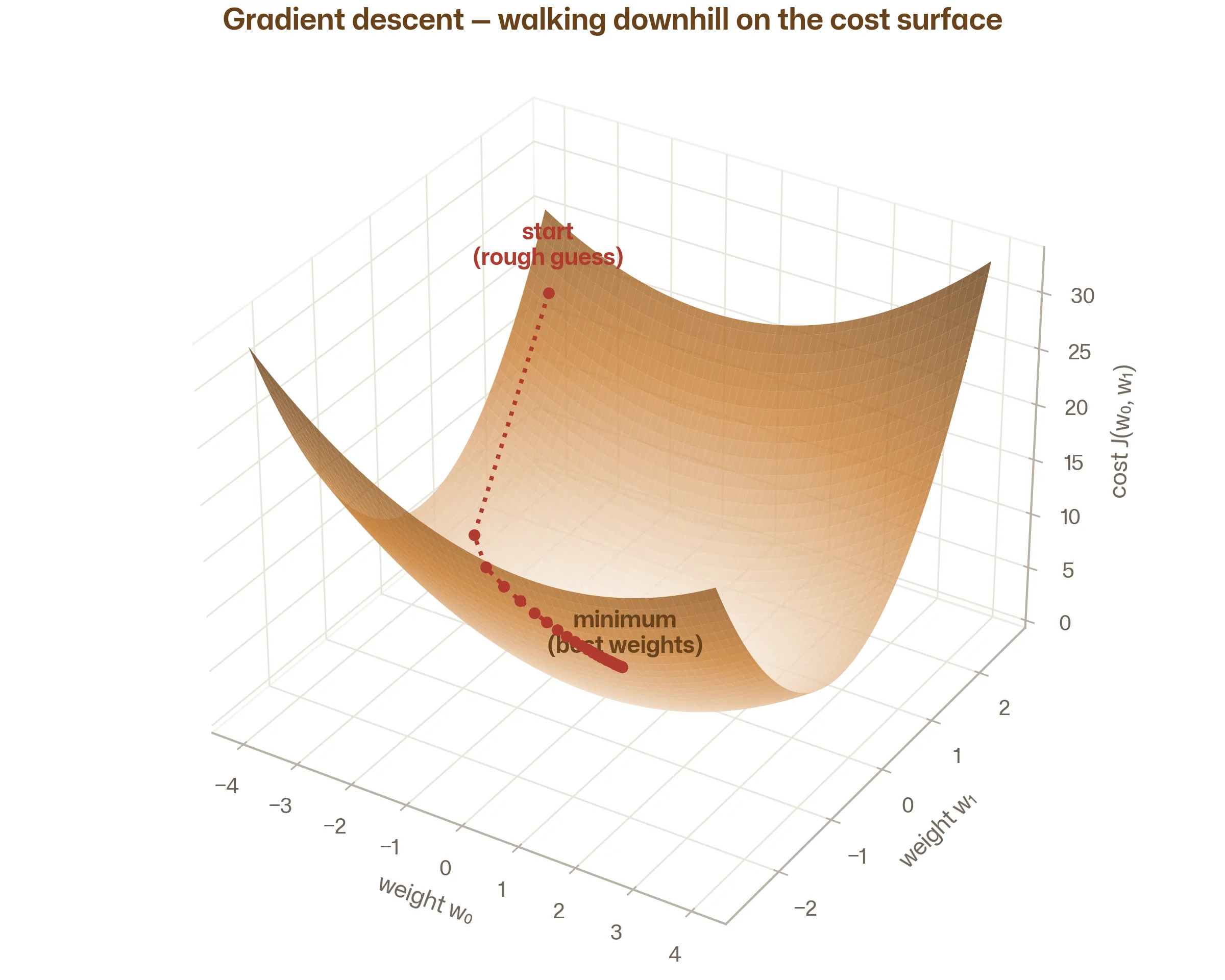
Gradient descent — the iterative approach. Start with random weights. Calculate the cost. Then nudge each weight slightly in the direction that reduces the cost. Repeat thousands of times until the cost stops improving.

If you've done any simulation work, gradient descent will feel familiar. It's the same principle as iterative FEA solvers that converge on a solution by reducing the residual at each step. You start with a rough answer, measure the error, adjust, and iterate until the error is small enough.

Gradient descent is slower than OLS for simple linear regression, so why learn it? Because gradient descent is how nearly every other ML algorithm trains. Neural networks, logistic regression, support vector machines — they all use variations of gradient descent to minimise their cost function. Understanding it here, with the simplest possible model, prepares you for everything that follows.

When linear regression works well

Linear regression is simple, but that doesn't mean it's weak. It's the right tool when:

The relationship is approximately linear. If doubling the feed rate roughly doubles the surface roughness (or at least the relationship is monotonic and smooth), linear regression will capture it well. Many engineering relationships are approximately linear within a limited operating range, even if they're non-linear across the full range.

You need interpretability. Each weight directly tells you how much each input affects the output. You can point to the model and say "feed rate has 3× the influence of depth of cut." Try doing that with a neural network.

You have limited data. Linear regression has very few parameters to learn (one weight per feature plus an intercept), so it can work well with small datasets — even 30–50 data points, if the relationship is genuinely linear. More complex models need more data to avoid overfitting.

You want a baseline. Even when you plan to use a more complex algorithm, start with linear regression. It gives you a reference point: if a Random Forest only performs 2% better than a simple linear model, the extra complexity might not be worth it. On the other hand, if it performs 30% better, you know the relationship is non-linear and the more complex model is justified.

When linear regression falls short

The relationship is non-linear. If surface roughness depends on feed rate in a complex, curved way — or if two variables interact (the effect of feed rate depends on spindle speed) — a straight line simply can't capture it. You'll see this as consistently high error on your test set. That's when it's time to move to algorithms like decision trees that handle non-linearity naturally.

You have many irrelevant features. Linear regression uses all features you give it, even unhelpful ones. It doesn't ignore irrelevant columns — it just assigns them small weights, which still add noise. Feature selection or regularisation (more on this in a moment) can help.

The data has outliers. Because the cost function squares the errors, a few extreme outliers can pull the entire line off course. One bad measurement can disproportionately affect the model. In engineering data, this is common — sensor glitches, mislabelled samples, or test specimens that failed for unrelated reasons.

A taste of what comes next: regularisation

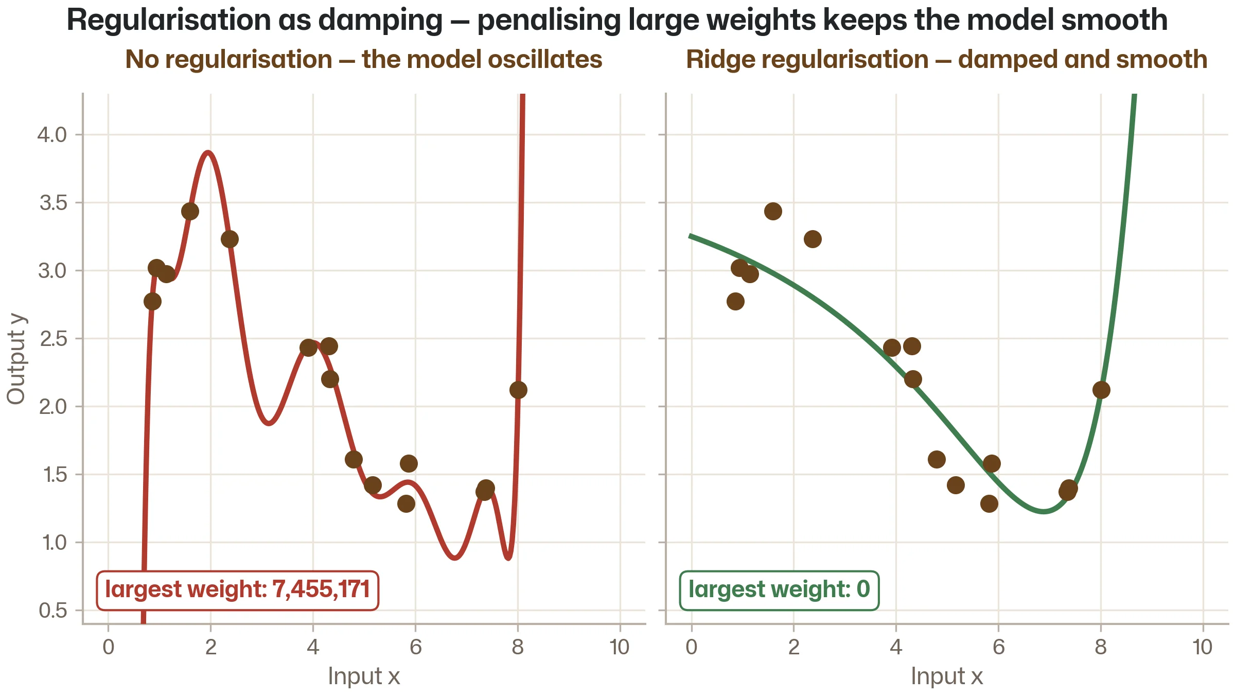
When you fit a model with many features, there's a risk of overfitting — the model starts fitting noise instead of real patterns. One elegant solution is regularisation: adding a penalty to the cost function that discourages overly large weights.

Think of it this way: if a weight is unnecessarily large, the model is overreacting to that feature. Regularisation adds a "tax" on large weights, forcing the model to find a solution that's both accurate and simple.

The two most common versions:

Ridge regression (L2) — adds a penalty proportional to the square of each weight. This shrinks all weights toward zero but never quite eliminates any. It's like adding damping to an oscillating system — it smooths out the response without removing any component entirely.

Lasso regression (L1) — adds a penalty proportional to the absolute value of each weight. This can shrink some weights all the way to zero, effectively removing those features from the model. It's automatic feature selection — the model decides which inputs matter and ignores the rest.

Both are still linear regression — they just add a constraint on how complex the solution can be. In scikit-learn, it's one line of code:

     
from sklearn.linear_model import Ridge, Lasso

ridge_model = Ridge(alpha=1.0)       # alpha controls penalty strength
lasso_model = Lasso(alpha=0.1)

ridge_model.fit(X_train, y_train)
predictions = ridge_model.predict(X_test)
                    

You'll meet regularisation again throughout this knowledge base. It's one of the central ideas in ML — the balance between fitting the data well and keeping the model simple enough to generalise. The full treatment is in the Overfitting and Underfitting article, next in this stage.

Linear regression in Python — five lines of code

Here's what a complete linear regression workflow looks like in scikit-learn. If you've read the previous articles in this knowledge base, every line should be recognisable — from the train/test split to the features and labels:

     
from sklearn.model_selection import train_test_split
from sklearn.linear_model import LinearRegression
from sklearn.metrics import mean_squared_error
import numpy as np

# Assume X = features table, y = labels column (already loaded)
# X might be: feed rate, spindle speed, depth of cut, tool wear
# y might be: surface roughness (Ra, µm)

# Step 1: Split into training and test sets
X_train, X_test, y_train, y_test = train_test_split(X, y, test_size=0.2, random_state=42)

# Step 2: Create and train the model
model = LinearRegression()
model.fit(X_train, y_train)

# Step 3: Predict on the test set
predictions = model.predict(X_test)

# Step 4: Measure how well the model performs
rmse = np.sqrt(mean_squared_error(y_test, predictions))
print(f"Root Mean Squared Error: {rmse:.3f}")

# Bonus: See which features matter most
for name, weight in zip(feature_names, model.coef_):
    print(f"  {name}: {weight:.4f}")
                    

That's the entire process. Load data, split, train, predict, evaluate. Every ML algorithm you'll learn in this knowledge base follows this same pattern — only the model creation line changes. For a Random Forest, you'd swap LinearRegression() for RandomForestRegressor(). For XGBoost, XGBRegressor(). The workflow stays the same.

The bonus section at the end — printing the weights — is where the engineering insight lives. Those weights tell you exactly how each process parameter contributes to the prediction. That's information you can take to a design review.

Logistic regression: the classification cousin

Despite having "regression" in the name, logistic regression is actually a classification algorithm. It's the classification equivalent of linear regression, and it's worth mentioning here because the name trips people up.

Logistic regression works like this: it calculates a linear combination of the inputs (just like linear regression), but then passes the result through a function that squashes the output to a value between 0 and 1. That output is interpreted as a probability — the probability that the data point belongs to one of two categories.

If the probability is above your threshold (say 50%), the model predicts "fail." Below the threshold, it predicts "pass."

The name is confusing, but the key takeaway is simple: linear regression predicts a number, logistic regression predicts a probability (which becomes a category). Same core idea, different output type. Same interpretable weights, same simplicity, same strengths and limitations.

You'll encounter logistic regression again when we cover classification algorithms in more detail. For now, just know it exists, it's useful, and the name is misleading.

Key takeaways

Linear regression finds the best straight line (or hyperplane) through your data. It's the simplest ML algorithm, but don't mistake simplicity for weakness — it's interpretable, fast, and works well when relationships are approximately linear.

The cost function is how any model measures its error. For linear regression, it's the mean squared error — the average of the squared differences between predictions and actual values. Every ML algorithm has a cost function. Training the model means minimising it.

Gradient descent is the universal training method. Start with random weights, measure the cost, adjust to reduce it, repeat. This iterative process is how nearly every ML algorithm learns — understanding it here prepares you for everything ahead.

Regularisation prevents overfitting. Ridge and Lasso add a penalty on large weights, keeping the model from overreacting to noise. Think of it as damping in a dynamic system.

Start with linear regression as a baseline. Even if you plan to use something more complex, a linear model gives you a reference point and immediate insight into which features matter.