What Is a Random Forest?

The problem with a single tree

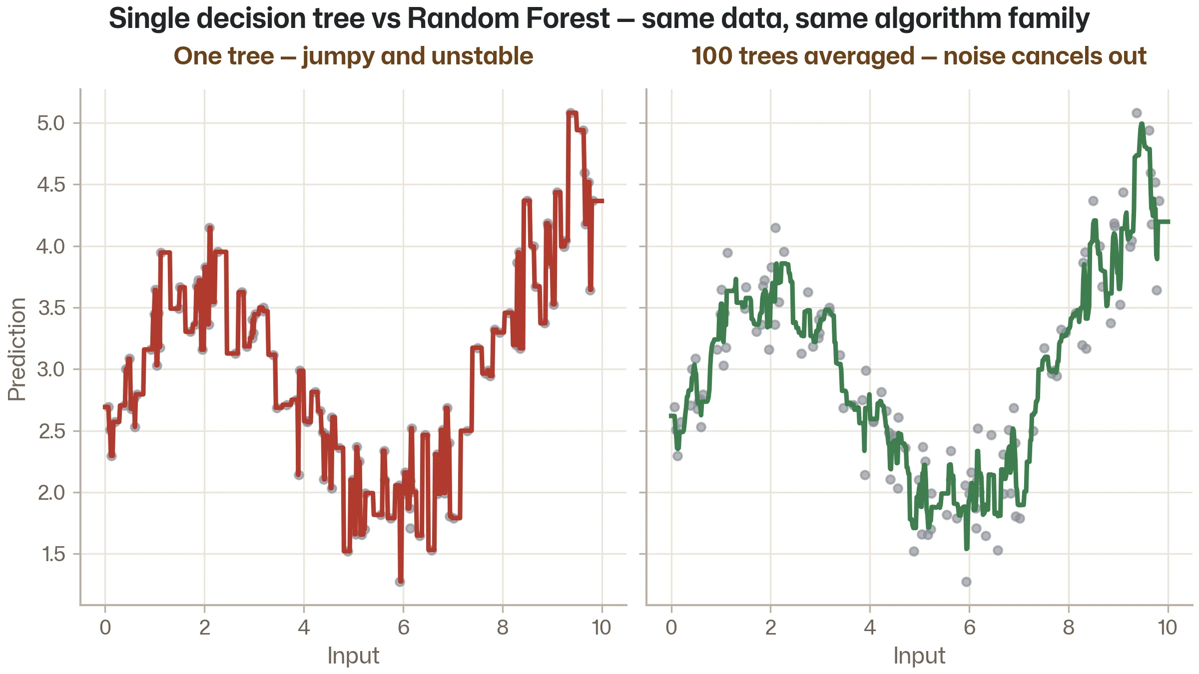
In the previous article, you saw that decision trees have a fundamental weakness: they overfit easily. A single tree, left unconstrained, will memorise the training data. Even with careful depth control, a single tree is unstable — change a few data points in the training set, and you can get a completely different tree with different splits and different predictions.

This instability isn't just a theoretical concern. Imagine you're building a model to predict weld quality, and you train a decision tree. Now imagine you collect 10 more data points and retrain. The new tree might split on different features, in a different order, and produce noticeably different predictions. That's not the kind of reliability an engineer can take to a design review.

The solution is elegant: don't rely on one tree. Train many trees, and let them vote.

That's a Random Forest.

How a Random Forest works

The idea is surprisingly simple. There are only two ingredients:

Ingredient 1: Bagging (training on different data subsets)

Instead of training one tree on all 500 data points, you create 100 different training sets by randomly sampling with replacement from the original data. Each sample is the same size as the original (500 points), but because you're sampling with replacement, each one contains some duplicate rows and is missing some original rows. On average, each sample contains about 63% of the unique original data points.

This technique is called bootstrap aggregating, or "bagging" for short. Each tree gets a slightly different view of the data, so each tree learns slightly different patterns. Some trees will pick up on one relationship, others on another.

Ingredient 2: Feature randomisation (asking different questions)

Here's the second trick: at each split in each tree, the algorithm doesn't consider all available features. Instead, it randomly selects a subset of features and picks the best split from only that subset.

Why? Because without this step, all your trees would look nearly identical. If melt temperature is the best overall split, every tree would start by splitting on melt temperature, and you'd just have 100 copies of roughly the same tree. Feature randomisation forces the trees to explore different splitting strategies, creating genuine diversity.

The prediction: let them vote

For classification, each tree casts a vote for a category, and the forest returns the majority vote. If 73 trees say "good" and 27 say "defective," the forest predicts "good" with 73% confidence.

For regression, each tree predicts a number, and the forest returns the average. If 100 trees predict stress values ranging from 230 to 260 MPa, the forest prediction is the mean — say, 247 MPa.

This is the same principle behind taking multiple measurements and averaging them to reduce uncertainty. One measurement might be off. The average of 100 independent measurements is reliable.

Why Random Forests are so popular

Random Forests have been a workhorse of applied ML for over two decades, and for good reason. Here's what makes them a natural first choice for engineering problems:

They're hard to get wrong. Unlike many algorithms, Random Forests work well out of the box with minimal tuning. The default settings in scikit-learn are sensible for most problems. You can spend hours fine-tuning hyperparameters, but the defaults will usually get you 90% of the way there.

They resist overfitting naturally. This is the big one. A single decision tree overfits easily, but the averaging effect in a Random Forest dramatically reduces overfitting. Adding more trees almost never hurts — the model just gets more stable. This is the opposite of increasing tree depth, where more complexity eventually destroys test performance.

They handle messy real-world data gracefully. Mixed feature types (continuous and categorical), missing values (in some implementations), non-linear relationships, feature interactions — Random Forests handle all of these without extensive preprocessing. For engineering datasets that come straight from a production database with inconsistent units and missing sensor readings, this robustness is invaluable.

They give you feature importance. Just like a single tree, a Random Forest tells you which features matter most — but averaged across 100+ trees, the importance scores are much more stable and reliable. We saw feature importance in the Decision Tree article; in a Random Forest, it's the same concept with less noise.

They scale well. Each tree is independent, so they can be trained in parallel. Training 100 trees on a modern laptop takes seconds to minutes for typical engineering datasets.

Random Forest vs single decision tree: a comparison

Let's make the improvement concrete. Here's what typically happens when you compare a single tree to a Random Forest on the same engineering dataset:

	Single decision tree (depth 5)	Random Forest (100 trees, depth 5 each)
Training accuracy	89%	92%
Test accuracy	83%	88%
Overfitting gap	6%	4%
Stability	Changes significantly if you add or remove a few data points	Nearly identical predictions across different data samples
Feature importance	Noisy — depends on which splits happened first	Stable — averaged across 100 trees

The Random Forest doesn't just perform better — it performs more reliably. The gap between training and test accuracy is smaller (less overfitting), and the predictions are stable across different data samples (less variance).

This is the wisdom-of-the-crowd effect. Any individual tree might be wrong about a specific data point, but the majority of trees will usually get it right. The errors of individual trees are random and uncorrelated (because each tree was trained on different data with different feature subsets), so they cancel out when you average.

Out-of-bag evaluation: free cross-validation

Remember that each tree is trained on a bootstrap sample that contains about 63% of the original data? That means about 37% of the data wasn't used to train that particular tree. These "left out" samples are called out-of-bag (OOB) samples.

Here's the clever part: for each data point, you can collect predictions from only the trees that didn't see that data point during training. This gives you a performance estimate that's very similar to cross-validation — but it comes for free, as a byproduct of the bagging process. No additional computation, no separate validation set needed.

In scikit-learn, you just set oob_score=True:

     
from sklearn.ensemble import RandomForestRegressor

model = RandomForestRegressor(n_estimators=100, oob_score=True, random_state=42)
model.fit(X_train, y_train)

print(f"OOB R² score: {model.oob_score_:.3f}")
                    

This is particularly useful when your dataset is small and you can't afford to set aside a large test set. The OOB score gives you an honest estimate of generalisation performance without sacrificing training data.

When Random Forests are the right choice

As your first model on a new problem. Before trying anything fancier, train a Random Forest. It gives you a strong baseline, reliable feature importances, and a performance level that more complex models need to beat to justify their added complexity.

When you need robustness over peak performance. Random Forests are rarely the absolute best performer on any single dataset, but they're consistently among the top performers across virtually all datasets. If you need a model that works well without extensive tuning and won't embarrass you with a bizarre prediction, Random Forest is a safe bet.

When interpretability matters. Feature importance from a Random Forest is a powerful and understandable tool. You can tell a process engineer "melt temperature and injection pressure account for 70% of the model's prediction power" and they can act on it.

When you have limited ML experience. The learning curve is gentle. There are few hyperparameters that matter much, the algorithm is forgiving of suboptimal settings, and it works well on the kinds of tabular data engineers typically have.

When to consider something else

When you need maximum accuracy on a competition-style benchmark. Gradient boosting methods (XGBoost, LightGBM) typically squeeze out a few more percentage points of accuracy. We'll cover these in the next article.

When you have very few samples. Random Forests need enough data to create diverse bootstrap samples. With fewer than 50–100 data points, you might not have enough for bagging to add value over a single, carefully tuned model.

When training speed is critical and your dataset is very large. For datasets with millions of rows, Random Forests can become slow because each tree sees the full dataset size (via bootstrap). Gradient boosting methods can be more efficient in this regime.

When you need uncertainty estimates. Random Forests give you a single prediction (the average or vote). They don't naturally tell you how confident that prediction is. For applications where you need uncertainty bounds — like safety-critical surrogate models — Gaussian Process Regression (covered in Stage 4) is a better choice.

Random Forest in Python

Here's a complete example, following the same pattern as every previous article:

     
from sklearn.ensemble import RandomForestRegressor
from sklearn.model_selection import train_test_split
from sklearn.metrics import mean_squared_error
import numpy as np

# Assume X = features, y = labels
# Example: predicting injection moulding shrinkage from process parameters
X_train, X_test, y_train, y_test = train_test_split(X, y, test_size=0.2, random_state=42)

# Train a Random Forest
model = RandomForestRegressor(
    n_estimators=100,    # number of trees (more is generally better)
    max_depth=10,        # limit depth to reduce overfitting
    random_state=42
)
model.fit(X_train, y_train)

# Evaluate
predictions = model.predict(X_test)
rmse = np.sqrt(mean_squared_error(y_test, predictions))
print(f"RMSE: {rmse:.3f}")

# Feature importance — stable across 100 trees
for name, imp in sorted(zip(feature_names, model.feature_importances_), key=lambda x: -x[1]):
    print(f"  {name}: {imp:.3f}")
                    

Notice how similar this is to the linear regression code from two articles ago. The only line that changed is the model creation. The workflow — split, train, predict, evaluate, inspect feature importances — is identical. That's the power of scikit-learn's consistent API: learn the pattern once, apply it to any algorithm.

The two hyperparameters worth paying attention to:

• n_estimators (number of trees): more is generally better, up to a point of diminishing returns. 100 is a solid starting point. 500 is rarely necessary for engineering-sized datasets.
• max_depth (depth of each tree): controls the complexity of individual trees. Start with 10–15 and adjust based on the training vs test gap.

Key takeaways

A Random Forest is a collection of decision trees that vote. Each tree is trained on a different random subset of the data, using a random subset of features at each split. The final prediction is the average (regression) or majority vote (classification).

Averaging diverse trees reduces overfitting. Individual trees may memorise noise, but because each tree memorises different noise, the average cancels it out. The real signal — shared across most trees — survives.

Random Forests are hard to get wrong. Minimal tuning required, robust to messy data, and consistently strong performance. They're the safest first choice for most engineering ML problems.

Feature importance is more reliable with a forest. Averaged across 100+ trees, importance scores are stable and actionable — unlike the noisy single-tree version.

Random Forests are the stepping stone to gradient boosting. They use independent trees that vote. The next article covers XGBoost, which uses sequential trees that correct each other's mistakes — a more powerful but more complex approach.