What Is a Decision Tree?

You've used decision trees your entire career

You've just never called them that.

Every troubleshooting flowchart you've followed — "Is the motor running? No → check power supply. Yes → is there vibration? Yes → check bearing alignment" — is a decision tree. A series of questions, asked in sequence, where each answer narrows down the diagnosis until you reach a conclusion.

ML decision trees work exactly the same way. The algorithm looks at your data and builds a flowchart of yes/no questions that splits the data into groups. At the end of each path through the tree, it makes a prediction — either a number (regression) or a category (classification).

The difference from a hand-built flowchart: you don't write the questions. The algorithm figures out which questions to ask, in which order, by analysing the data. It determines which feature to split on, what threshold to use, and how deep to go — all automatically, all optimised to make the most accurate predictions possible.

How the algorithm builds the tree

The algorithm builds the tree from the top down, one question at a time. At each step, it asks: which question splits the data most usefully?

Here's the process, step by step:

Step 1: Look at all the data. The algorithm starts with your entire training set — say 500 injection moulding cycles, each with process parameters (features) and a quality result (label: good or defective).

Step 2: Find the best first question. It tries every possible split — every feature, at every possible threshold value. "Is melt temperature > 195°C?" "Is injection pressure > 85 bar?" "Is cooling time > 12 seconds?" For each candidate split, it measures how well it separates the data into groups that are more "pure" (mostly good or mostly defective).

Step 3: Split the data. The best question becomes the first node of the tree. The data is divided into two branches: the samples that answered "yes" and those that answered "no."

Step 4: Repeat on each branch. For each subset, the algorithm again finds the best question to split it further. And then again, and again — creating a deeper and deeper tree.

Step 5: Stop when a stopping condition is met. The tree stops growing when it reaches a maximum depth, when the groups are already pure enough, or when further splitting wouldn't improve predictions significantly.

The result is a tree of questions that you can read from top to bottom. Every prediction is a traceable path through the tree — you can point to exactly which questions led to the result. No black box. No mysterious weights. Just a sequence of if/then rules.

How does the algorithm decide what "best split" means?

The algorithm needs a way to measure the quality of a split. For classification, the most common measure is Gini impurity — a number between 0 and 1 that measures how mixed a group is.

A group that's 100% defective parts has a Gini impurity of 0 — perfectly pure. A group that's 50% good and 50% defective has the highest Gini impurity — maximally mixed. The algorithm chooses the split that creates the purest subgroups.

For regression trees, the algorithm typically uses the mean squared error of each subgroup — the same cost function from the Linear Regression article. It splits the data in a way that minimises the prediction error within each resulting group.

A concrete example: injection moulding quality

Let's walk through a simplified example. You have data from 200 injection moulding cycles, with four features and a binary label (good/defective).

The algorithm might build a tree like this:

     
Is melt temperature > 210°C?
├── YES → Is injection pressure < 70 bar?
│         ├── YES → Predict: DEFECTIVE (18/20 defective)
│         └── NO  → Is cooling time > 15s?
│                   ├── YES → Predict: GOOD (45/48 good)
│                   └── NO  → Predict: DEFECTIVE (12/15 defective)
└── NO  → Is cycle time > 25s?
          ├── YES → Predict: DEFECTIVE (8/10 defective)
          └── NO  → Predict: GOOD (95/107 good)
                    

Read this like a flowchart. For a new moulding cycle with melt temperature 205°C, injection pressure 82 bar, and cycle time 22 seconds, you'd follow the path: temperature not > 210°C → NO → cycle time not > 25s → NO → predict GOOD.

Notice what the tree is telling you in engineering terms:

• High melt temperature combined with low injection pressure is a recipe for defects
• Within the high-temperature group, sufficient cooling time can compensate
• At lower temperatures, only excessively long cycle times cause problems

Decision trees and overfitting: the killer demo

This is the moment the Overfitting and Underfitting article promised. Decision trees make overfitting visible in a way no other algorithm can, because you can literally see the tree memorising the data.

An unpruned tree memorises everything

If you let a decision tree grow without any limits, it will keep splitting until every single training sample has its own leaf. A dataset with 200 data points? The tree creates 200 leaves — one custom rule for each row. Training accuracy: 100%. The tree didn't learn patterns; it built a lookup table.

Now test this tree on new data. The performance collapses. All those hyper-specific rules — "if temperature is exactly 203.7°C and pressure is exactly 81.3 bar" — don't match any new data points precisely. The tree is forced to make predictions based on rules that were tuned to individual quirks in the training set.

Pruning: controlling complexity

The fix is to limit how deep the tree can grow — a process called pruning. By setting a maximum depth, you force the tree to find rules that apply to groups of data points rather than individual ones. The tree captures the general patterns and ignores the noise.

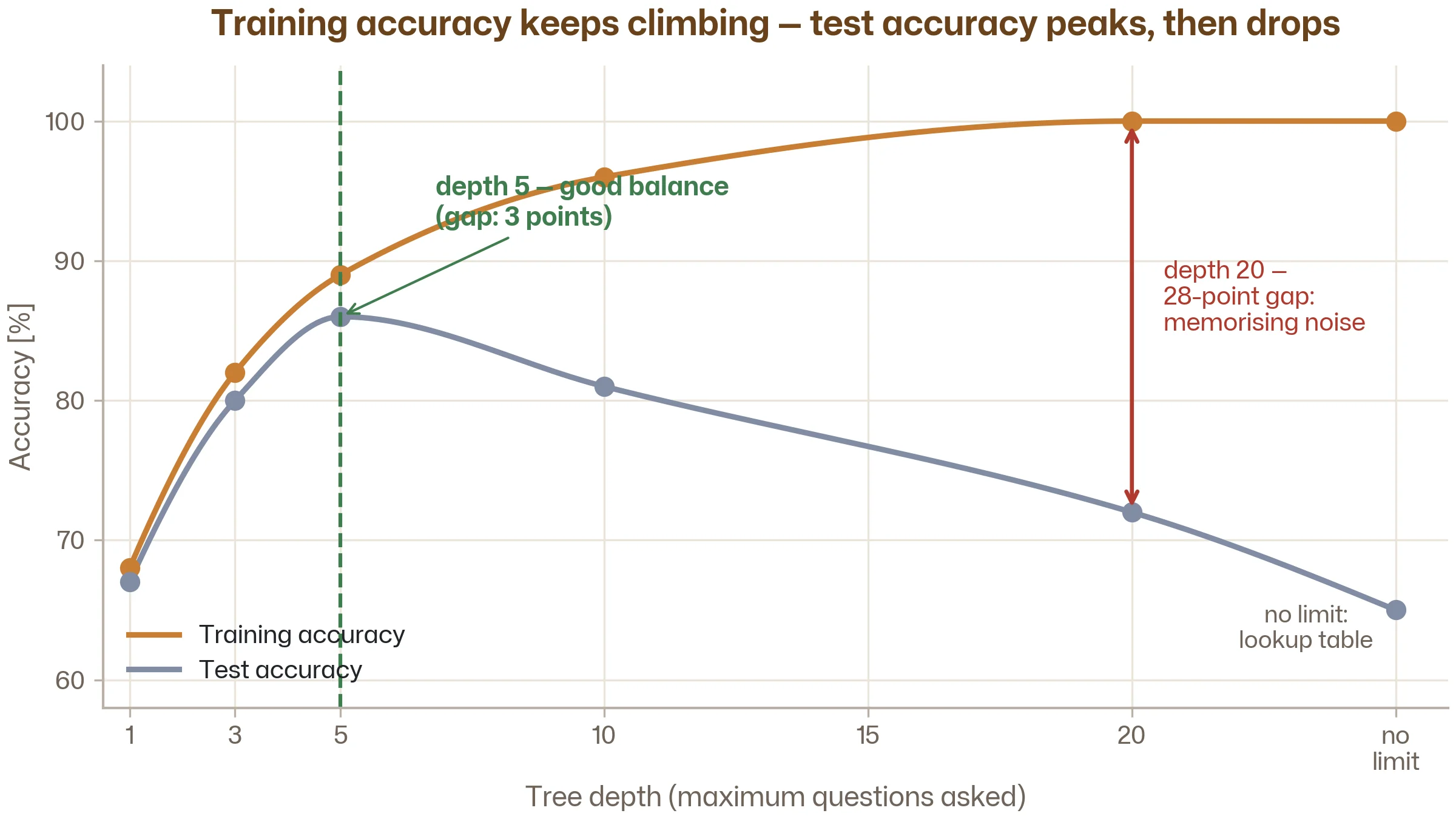
Here's what happens as you increase tree depth on a typical engineering dataset:

Tree depth	Training accuracy	Test accuracy	What's happening
1	68%	67%	Underfitting — one question isn't enough
3	82%	80%	Starting to capture real patterns
5	89%	86%	Good balance — real patterns captured
10	96%	81%	Starting to overfit — gap appearing
20	100%	72%	Severe overfitting — memorising noise
No limit	100%	65%	Total memorisation — lookup table

Look at the gap between training and test accuracy. At depth 5, it's only 3 percentage points — the model generalises well. At depth 20, the gap is 28 points — classic overfitting.

This table is the bias-variance trade-off in action. Shallow trees have high bias (too simple) but low variance (stable across datasets). Deep trees have low bias (can capture complex patterns) but high variance (sensitive to the specific training data). Somewhere in the middle is the sweet spot.

Decision trees for regression

Everything above used classification as an example, but decision trees work for regression too. Instead of predicting a category at each leaf, a regression tree predicts a number — typically the average of all training samples that ended up in that leaf.

For example, a regression tree predicting surface roughness might look like:

     
Is feed rate > 0.15 mm/rev?
├── YES → Is depth of cut > 2.5 mm?
│         ├── YES → Predict: Ra = 3.2 µm (average of 35 samples)
│         └── NO  → Predict: Ra = 1.8 µm (average of 42 samples)
└── NO  → Is spindle speed < 1200 rpm?
          ├── YES → Predict: Ra = 1.4 µm (average of 58 samples)
          └── NO  → Predict: Ra = 0.9 µm (average of 65 samples)
                    

The tree has divided the feature space into four regions, each with its own predicted roughness value. It's a piece-wise constant model — the predicted value is flat within each region and jumps at the boundaries.

This is fundamentally different from linear regression, which fits a smooth surface through the data. A regression tree creates rectangular regions with flat predictions. Neither is "better" — they have different strengths. Linear regression captures smooth trends. Trees capture sharp thresholds and interactions. Real engineering data often has both.

Why decision trees matter (even if you end up using something else)

You might be wondering: if decision trees overfit easily and make piece-wise constant predictions, why learn them at all? Three reasons:

1. They're the building block of the most powerful algorithms. Random Forest, XGBoost, LightGBM, CatBoost — the algorithms that dominate tabular data competitions and real-world engineering applications — are all built from decision trees. Understanding a single tree is essential to understanding why forests and boosted ensembles work so well. We'll cover these in the next two articles.

2. They're the best teaching tool for overfitting. No other algorithm makes overfitting as visible and intuitive. The depth-vs-accuracy curve you just saw is something you can reproduce in 10 lines of Python, and it cements the bias-variance trade-off in a way that no amount of theory can match.

3. They're genuinely useful on their own for interpretability. When you need a model that a quality engineer, a regulator, or a shop-floor operator can understand and verify, a shallow decision tree (depth 3–5) is unbeatable. You can print it, trace any prediction, and check whether the rules make physical sense. Try doing that with a neural network.

Decision trees in Python

Here's a complete example — training a classification tree with controlled depth:

     
from sklearn.tree import DecisionTreeClassifier, plot_tree
from sklearn.model_selection import train_test_split
from sklearn.metrics import accuracy_score
import matplotlib.pyplot as plt

# Assume X = features, y = labels (good/defective)
X_train, X_test, y_train, y_test = train_test_split(X, y, test_size=0.2, random_state=42)

# Train a tree with limited depth to prevent overfitting
model = DecisionTreeClassifier(max_depth=5, random_state=42)
model.fit(X_train, y_train)

# Evaluate
train_acc = accuracy_score(y_train, model.predict(X_train))
test_acc = accuracy_score(y_test, model.predict(X_test))
print(f"Training accuracy: {train_acc:.1%}")
print(f"Test accuracy:     {test_acc:.1%}")

# Visualise the tree — this is the magic moment
plt.figure(figsize=(20, 10))
plot_tree(model, feature_names=feature_names, class_names=["Good", "Defective"],
          filled=True, rounded=True, fontsize=10)
plt.tight_layout()
plt.savefig("decision_tree.png", dpi=150)
plt.show()
                    

Notice max_depth=5 — that's the overfitting control. Try changing it to 3, 10, and None (unlimited) and watch the gap between training and test accuracy grow. That experiment, on your own data, is worth more than reading ten articles about overfitting.

The plot_tree line at the end is what makes decision trees special. You get a full visual of every rule the model learned. No other algorithm gives you this level of transparency.

Feature importance: a free bonus

Decision trees automatically tell you which features matter most. Every time a feature is used for a split, it contributes to reducing the impurity (or error) in the data. Features used at the top of the tree — where splits affect the most data — are the most important.

     
# Get feature importances
importances = model.feature_importances_

# Print them, sorted by importance
for name, imp in sorted(zip(feature_names, importances), key=lambda x: -x[1]):
    print(f"  {name}: {imp:.3f}")
                    

This might output something like:

     
  melt_temperature: 0.42
  injection_pressure: 0.28
  cooling_time: 0.19
  cycle_time: 0.11
                    

Now you know: melt temperature is the dominant driver of quality in this process, followed by injection pressure. This is the kind of insight that leads to process improvement actions — and it came for free, as a byproduct of training the model.

Feature importance becomes even more powerful with Random Forests and XGBoost, where it's averaged across hundreds of trees for a more stable estimate. And when you need to explain individual predictions (not just global importance), SHAP takes this further — we'll cover that in Stage 4.

Key takeaways

A decision tree is a flowchart of yes/no questions. The algorithm builds it automatically by finding the splits that best separate the data. You can read, trace, and verify every prediction.

Trees make overfitting visible. An unlimited tree memorises the training data. A shallow tree finds general rules. The depth-vs-accuracy curve is the single best demonstration of the bias-variance trade-off.

Control complexity with tree depth. max_depth is the most important setting. Start shallow (3–5) and increase carefully, monitoring the gap between training and test performance.

Trees are the foundation for the most powerful algorithms. Random Forest, XGBoost, and other ensemble methods are all built from decision trees. Understanding one tree is the key to understanding them all.

Feature importance comes for free. The tree automatically ranks which inputs matter most — actionable engineering insight as a byproduct of making predictions.