The concept that separates beginners from practitioners
If you only learn one thing from this entire knowledge base, make it this.
Every ML model faces a fundamental tension: fit the training data well enough to capture real patterns, but not so well that it captures noise, quirks, and coincidences that won't repeat in new data.
Get this balance wrong in one direction, and your model is too simple — it misses real relationships in the data. Get it wrong in the other direction, and your model is too complex — it memorises the specific dataset it was trained on and falls apart on anything new.
These two failure modes have names:
The two failure modes
Underfitting: the model is too simple to capture the real patterns. It performs poorly on the training data and on new data. It hasn't learned enough.
Overfitting: the model is too complex and has memorised noise in the training data. It performs brilliantly on training data but poorly on new data. It has learned too much — including things that aren't real.
This isn't just an ML problem. Engineers deal with this trade-off constantly, under different names. You've seen it in curve fitting, in simulation, and in experimental design. ML just makes it explicit and gives you tools to manage it.

An analogy every engineer understands
Imagine you're fitting a curve to experimental data from a tensile test — stress versus strain for a new alloy, measured on 20 specimens.
The underfitting version: you fit a straight line. It captures the elastic region reasonably well, but completely misses the yield point, the strain hardening, and the necking behaviour. The model is too simple for the data. It can't represent the real physics.
The good fit version: you fit a sensible model — maybe a Ramberg-Osgood equation or a well-chosen polynomial. It captures the elastic region, the yield transition, and the strain hardening. It doesn't hit every data point exactly, but it follows the trend. The small gaps between the curve and the points? That's measurement noise, and you want the model to ignore it.
The overfitting version: you fit a 19th-degree polynomial that passes through all 20 data points perfectly. Zero error on the training data. But look at what happens between the data points: the curve oscillates wildly, predicting negative stress and physically impossible behaviour. If you use this curve to predict the stress at a strain value you didn't test, the prediction will be nonsensical.
The core lesson
The overfitted curve has zero training error but is completely useless for prediction. The good fit has some training error but is actually trustworthy. A small amount of training error is not just acceptable — it's desirable. A model that fits the training data too perfectly is almost certainly memorising noise.
How to detect overfitting
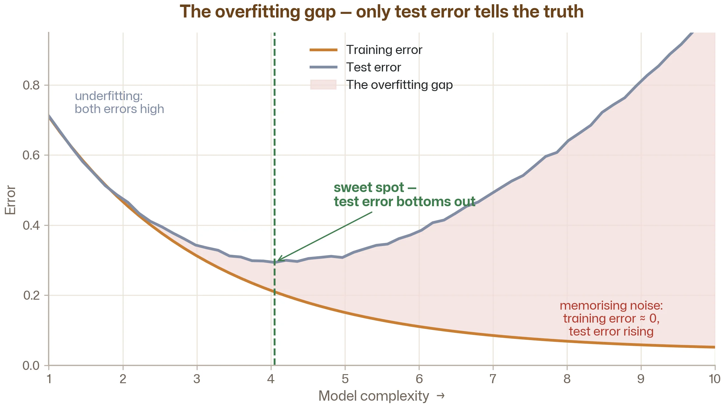
This is where the train/test split you learned in Stage 1 becomes essential. The signature of overfitting is a gap between training performance and test performance:
| Training error | Test error | Diagnosis | |
|---|---|---|---|
| Underfitting | High | High | Model too simple |
| Good fit | Low | Low (similar to training) | Model is appropriate |
| Overfitting | Very low | Much higher than training | Model too complex |
If your model scores 98% on training data but only 72% on test data, it's overfitting. The 26-point gap tells you it memorised the training set rather than learning generalisable patterns.
This is why you never evaluate on training data alone — a point we made in the Training Data vs Test Data article. Training error will always look good (or even perfect) for a sufficiently complex model. Only test error tells you the truth.
The bias-variance trade-off
Behind overfitting and underfitting lies a deeper concept called the bias-variance trade-off. You don't need to memorise the maths, but understanding the intuition helps you make better modelling decisions.
Bias is the error from overly simplistic assumptions. A linear model applied to a curved relationship has high bias — it's systematically wrong because it can't represent the true pattern. High bias → underfitting.
Variance is the error from being too sensitive to the specific training data. A wildly flexible model might fit one training set perfectly but produce a completely different curve on a different training set drawn from the same process. High variance → overfitting.
The trade-off: reducing bias (making the model more flexible) tends to increase variance, and vice versa. A simple model has high bias but low variance. A complex model has low bias but high variance. The goal is to find the sweet spot where the total error (bias + variance) is minimised.
The engineering analogy
Think of a PID controller. Very aggressive gains (high Kp) respond quickly to setpoint changes (low bias) but oscillate and overshoot with every disturbance (high variance). Conservative gains give a sluggish but stable response (high bias, low variance). You tune the controller to find the best compromise for your specific system. Model complexity works the same way.
What controls model complexity?
Different algorithms have different "knobs" that control how complex the model can become. Here are the ones you'll encounter most often:
For linear regression: the number of features. Adding more features (especially polynomial features or interaction terms) increases complexity. Regularisation (Ridge, Lasso) reduces it by penalising large weights, as we covered in the previous article.
For decision trees: the depth of the tree. A tree with depth 2 can only ask two questions — very simple. A tree with depth 20 can carve the data into millions of tiny regions — very complex and almost certainly overfitting. You'll see this dramatically when we cover decision trees in the next article.
For random forests and XGBoost: the number of trees, the depth of each tree, the minimum number of samples in each leaf, and several other settings. These are all hyperparameters — settings you choose before training, as opposed to the weights the model learns during training. We'll explore hyperparameter tuning in Stage 3.
For neural networks: the number of layers, the number of neurons per layer, and the training duration. More layers and neurons mean more capacity to fit complex patterns — and more risk of overfitting.
The key principle: more complexity is not always better. A model with 1,000 parameters trained on 200 data points will almost certainly overfit. A model with 5 parameters on the same data might underfit. Somewhere in between is the right balance, and it depends on your specific data.

Practical strategies to prevent overfitting
Overfitting is far more common than underfitting in practice. Here are the tools you have to fight it:
1. Get more data
The single most effective defence. With more data, the model has a harder time memorising individual quirks because there are too many examples to memorise — it's forced to learn the general pattern instead.
This isn't always possible in engineering (simulations are expensive, tests take time), but when it is, more data almost always helps more than a fancier algorithm.
2. Use a simpler model
If your decision tree has depth 20 and it's overfitting, try depth 5. If your polynomial regression has 8th-degree features, try 2nd-degree. Reducing model complexity is the most direct way to reduce overfitting.
The question is always: does the simpler model still capture the real pattern? If yes, prefer it. If the simpler model clearly underfits, you need to find the middle ground.
3. Regularisation
We introduced this in the Linear Regression article. Ridge and Lasso penalise overly complex solutions by adding a cost for large weights. The model is forced to find a solution that fits the data and keeps the weights small — a built-in preference for simplicity.
Regularisation exists for almost every algorithm, not just linear regression. For decision trees, limiting the depth is a form of regularisation. For neural networks, dropout and weight decay serve the same purpose. The underlying principle is always the same: add a constraint that prevents the model from becoming more complex than the data justifies.
4. Cross-validation
Instead of relying on a single train/test split, cross-validation rotates through multiple splits and averages the results. This gives you a more reliable estimate of how well your model generalises and helps you detect overfitting more consistently. We'll cover this in detail in Stage 3.
5. Feature selection
Remove features that don't carry useful information. As we discussed in the Features and Labels article, irrelevant columns don't just waste computation — they give the model noise to memorise. Your engineering knowledge is invaluable here: you know which process parameters are physically relevant and which are just database artefacts.
Underfitting: the less glamorous problem
Overfitting gets all the attention, but underfitting is equally problematic — and often easier to fix.
Signs of underfitting:
- Training error is high (the model can't even fit the data it trained on)
- Training and test error are similar (both bad)
- The model's predictions are consistently off in a systematic way (always too high, or missing a clear curved relationship)
Fixes for underfitting:
- Use a more complex model. Switch from linear regression to a decision tree or random forest. The data might have non-linear patterns that a simple model can't capture.
- Add more features. Maybe the model doesn't have enough information. Engineering-derived features (ratios, interactions, rolling statistics) can help enormously.
- Add polynomial or interaction terms. For linear regression, including features like feed_rate² or feed_rate × spindle_speed lets the model capture non-linear relationships while remaining within the linear regression framework.
- Reduce regularisation. If you're using Ridge or Lasso, the penalty might be too strong, preventing the model from fitting real patterns. Try reducing the alpha parameter.
Overfitting with decision trees: a preview
The next article in this stage covers decision trees, and it's where overfitting becomes truly visible. A decision tree with no depth limit will create a separate rule for every single data point in the training set — achieving perfect training accuracy and terrible test accuracy. You can literally print the tree and see it memorising individual rows.
Then, when you limit the tree depth, you watch the test accuracy improve as the model is forced to find general rules instead of specific memorisations. It's the most visceral, convincing demonstration of overfitting in all of ML, and it makes the bias-variance trade-off tangible rather than theoretical.
That's the power of learning decision trees after understanding overfitting — you'll see the concept playing out in real time.
Key takeaways
Overfitting = the model learned the noise. It performs well on training data but poorly on new data. The gap between training and test performance is the telltale sign.
Underfitting = the model is too simple. It performs poorly on both training and test data. It hasn't captured the real patterns.
The bias-variance trade-off is the fundamental tension. Simpler models have high bias but low variance. Complex models have low bias but high variance. The sweet spot is in between, and it depends on your data.
You manage this trade-off through model complexity. Tree depth, number of features, regularisation strength, network size — these are all knobs that move you along the bias-variance spectrum.
More data is the best defence against overfitting. When you can't get more data, use regularisation, simpler models, feature selection, and cross-validation.
Every ML algorithm you'll ever use is subject to this trade-off. The specific knobs change, but the underlying principle is always the same. Master this concept, and you'll make better modelling decisions with any algorithm.
Frequently asked questions
Common questions about overfitting, underfitting, and model complexity.
Compare your model's performance on the training set versus a held-out test set. If training accuracy is much higher than test accuracy — say 97% vs 78% — the model is overfitting. The size of that gap is your diagnostic signal. A small gap (a few percentage points) is normal. A large gap (10+ points) means the model is memorising noise rather than learning generalisable patterns.
There's no universal number — it depends on the problem, the dataset size, and the noise in your data. As a rough guideline, a gap under 3–5 percentage points usually indicates a healthy model. A gap of 10+ points is a warning sign. What matters most is the trend: if increasing model complexity widens the gap without improving test performance, you've gone too far. Use the test error as your primary metric, not the training error.
A tiny amount of overfitting is practically unavoidable and not a concern. Any model that fits the data well will have slightly better training performance than test performance — that's normal. The problem starts when the gap becomes large and the test performance degrades. The goal isn't zero overfitting; it's finding the model complexity that maximises performance on unseen data.
Both are strategies to reduce overfitting, but they apply to different algorithms. Regularisation (Ridge, Lasso) adds a penalty to the cost function that discourages large weights — it's primarily used with linear models and neural networks. Pruning limits the depth or size of a decision tree, preventing it from growing complex enough to memorise the training data. They're different mechanisms, but the underlying idea is the same: constrain model complexity to improve generalisation.
No — the opposite approach is usually better. Start with a simple model (linear regression, shallow decision tree) to establish a baseline. If the simple model underfits, gradually increase complexity. This way you can see exactly when the model becomes "complex enough" and when extra complexity stops helping. Starting with the most complex model makes it harder to diagnose problems and often leads to overfitting that you then have to work backwards to fix.
Yes, though the risk varies. Random Forests are naturally resistant to overfitting — adding more trees generally doesn't hurt. However, very deep trees within the forest can still overfit, especially on small datasets. XGBoost is more susceptible: too many boosting rounds, a high learning rate, or overly deep trees can all lead to overfitting. That's why XGBoost relies on early stopping — it automatically halts training when the validation error stops improving.
Follow the learning path
This is article 2 in Stage 2: The Algorithms. Next up: decision trees — where overfitting becomes visible. Subscribe and we'll let you know when it's ready.
Subscribe to the newsletter