What Is Gradient Boosting (XGBoost)?

From voting to error correction

In the previous article, you learned that a Random Forest trains many trees independently and averages their predictions. Each tree gets a different random view of the data, and the averaging cancels out noise. It's a powerful idea — but it has a limitation.

Because each tree is trained independently, no tree knows what the other trees got wrong. Tree 47 doesn't know that tree 12 badly mispredicted the stress for short, thick beams. Tree 93 doesn't know that the whole forest consistently underestimates roughness at high feed rates. Each tree does its best in isolation, and you hope the average is good enough.

Gradient boosting takes a fundamentally different approach:

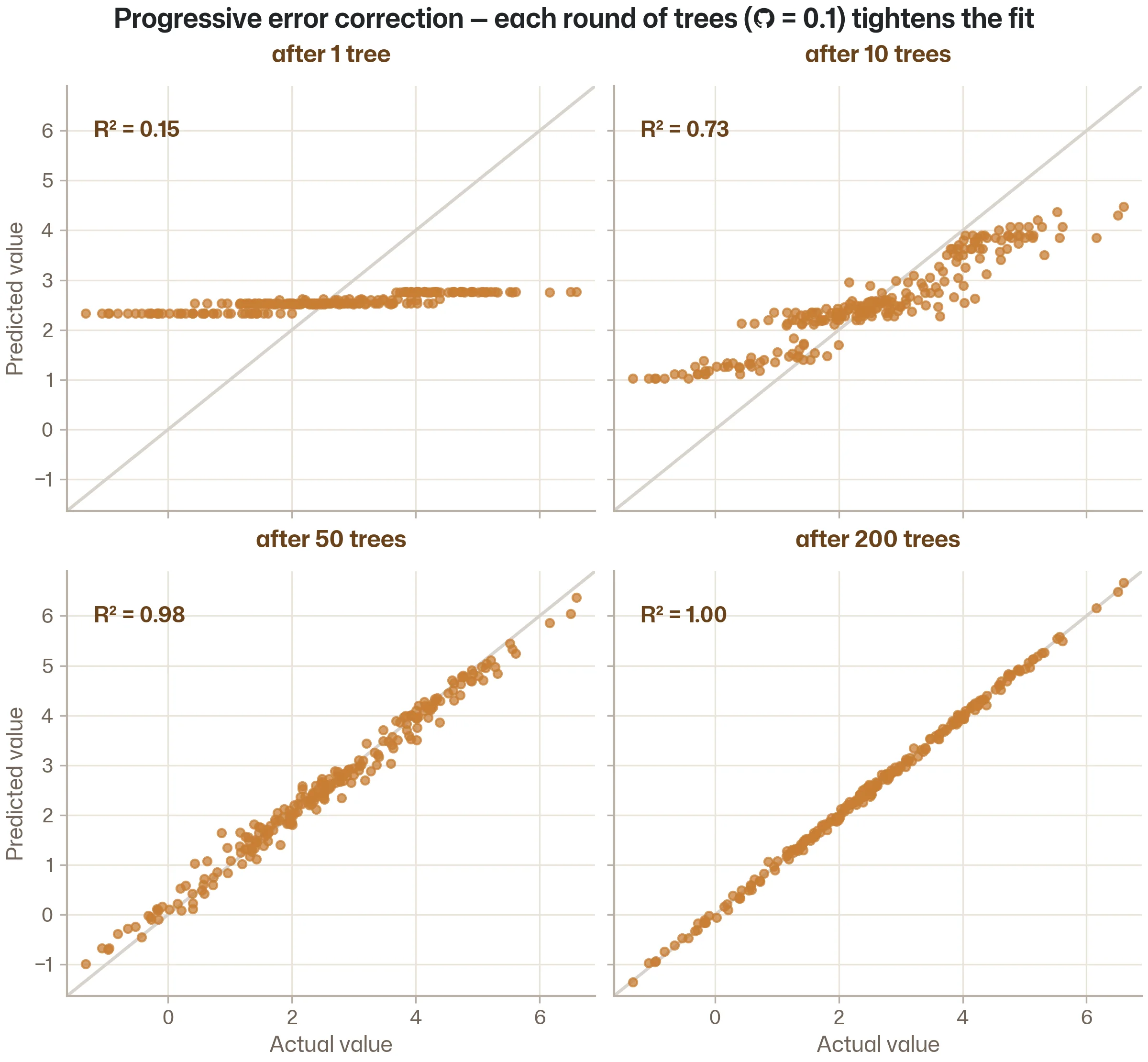
The first tree makes predictions. Some are good, some are off. The second tree doesn't start from scratch — it looks at where the first tree was wrong, and tries to fix those errors. The third tree corrects the remaining errors from the first two combined. And so on, for 100 or 500 or 1,000 rounds.

The result is a model that progressively zeroes in on the right answer, getting a little better with each tree. It's iterative refinement — a concept every engineer already trusts.

How gradient boosting works, step by step

Let's walk through the process with a concrete engineering example. You're predicting the shrinkage of injection-moulded parts from five process parameters, and you have 300 training samples.

Round 1: Train the first tree. A shallow tree (typically depth 3–6) makes predictions for all 300 samples. Some predictions are close, others are off. You calculate the residuals — the difference between the actual shrinkage and the predicted shrinkage for each sample.

Sample	Actual shrinkage	Tree 1 prediction	Residual (error)
A	2.1%	1.8%	+0.3%
B	1.5%	1.8%	−0.3%
C	3.2%	2.5%	+0.7%
D	1.9%	1.8%	+0.1%

Round 2: Train a second tree on the residuals. The second tree doesn't try to predict shrinkage directly. Instead, it tries to predict the errors of the first tree. It learns that sample C was badly underestimated, and finds a pattern: parts with high melt temperature and long cooling time tend to have residuals around +0.7%.

Round 3 and beyond: keep correcting. Each new tree predicts the remaining residuals from all previous trees combined. With each round, the residuals get smaller — the model is converging on the true relationship, a little bit at a time.

Final prediction: The final prediction is the sum of all trees' contributions:

Each tree contributes a small correction. No single tree needs to be accurate on its own — it just needs to improve the current combined prediction by a little bit.

The learning rate: how much to trust each correction

There's one crucial detail: each tree's contribution is multiplied by a learning rate (typically 0.01 to 0.3) before being added to the running total.

Why shrink each correction? Because trees make mistakes too, and you don't want to overcorrect. A learning rate of 0.1 means "only trust each correction at 10% strength." This makes the process more conservative and more robust — it takes more trees to converge, but the final result is better.

Think of it like adjusting a micrometer: you could crank it in large increments and risk overshooting, or advance it in small, careful steps and land precisely on the target. Gradient boosting chooses small steps. The learning rate controls the step size.

Why is it called "gradient" boosting?

The word "gradient" comes from the optimisation method used under the hood. Remember the cost function from the Linear Regression article? Gradient boosting uses the same idea: there's a cost function measuring the total error, and the algorithm uses the gradient (the mathematical slope of the cost function) to determine the direction in which each new tree should push the predictions.

"Gradient descent on the cost function, but instead of adjusting weights, you add a new tree at each step."

You don't need to understand the maths to use gradient boosting effectively. The practical takeaway: each tree is optimally aimed at reducing the remaining error, not just randomly trying to help. This directed correction is what makes gradient boosting more efficient than Random Forest — it converges on a good solution faster, with fewer trees.

XGBoost, LightGBM, CatBoost: the implementations

"Gradient boosting" is the general principle. The specific software packages you'll encounter are:

XGBoost (Extreme Gradient Boosting) — the most widely used implementation. It introduced several engineering improvements (parallel tree construction, built-in regularisation, efficient handling of missing values) that made gradient boosting practical for large datasets. XGBoost has won more Kaggle competitions than any other algorithm and is the standard recommendation for tabular data.

LightGBM (Light Gradient Boosting Machine) — Microsoft's implementation, optimised for speed on very large datasets. Uses a different tree-growing strategy (leaf-wise instead of level-wise) that can be faster and more accurate, but also more prone to overfitting on small datasets.

CatBoost (Categorical Boosting) — Yandex's implementation, with built-in support for categorical features (like material grade, machine ID, or shift). If your dataset has many categorical columns, CatBoost can handle them natively without one-hot encoding.

For most engineering problems with datasets under 100,000 rows, all three perform similarly. XGBoost is the safest default — it has the largest community, the most tutorials, and the most predictable behaviour. If you learn XGBoost, switching to LightGBM or CatBoost later takes minutes, not days.

XGBoost vs Random Forest: when does it matter?

Both algorithms use ensembles of decision trees. Both handle tabular data well. So when does the difference matter?

	Random Forest	XGBoost
Training approach	Independent trees, averaged	Sequential trees, each correcting errors
Default performance	Very good with minimal tuning	Slightly better, but needs more tuning
Overfitting risk	Low — adding more trees always helps	Higher — too many trees or a too-high learning rate will overfit
Tuning complexity	Few knobs, hard to go wrong	More knobs, more opportunity to optimise (and to mess up)
Missing values	Requires imputation in scikit-learn	Handles natively
Training speed	Fast (parallelisable)	Moderate (sequential by nature, though implementations parallelise internally)
Typical use	First model, baseline, "I need something reliable now"	Second model, when you want to push accuracy further

The practical advice: start with Random Forest. If you need better performance, switch to XGBoost and tune it. The performance difference is typically 1–5% on engineering datasets — meaningful for competitions, often irrelevant for real-world applications where the bottleneck is data quality, not algorithm choice.

That said, XGBoost is the algorithm cited in the NeurIPS paper we discussed earlier — the one that consistently outperforms neural networks on tabular data. When you read "tree-based models beat deep learning," XGBoost is usually the tree-based model doing the beating.

The key hyperparameters

XGBoost has many hyperparameters, but only a handful matter for most problems. Here are the ones to start with:

n_estimators (number of trees): how many sequential correction rounds. More trees means more refinement, but too many can overfit. Start with 100–500. Use early stopping (below) to find the right number automatically.

max_depth (tree depth): how deep each individual tree can grow. Gradient boosting typically uses shallower trees than Random Forest — depth 3–6 is common, compared to 10–15 for Random Forest. Shallow trees are "weak learners" that each contribute a small correction.

learning_rate (eta): how much each tree's contribution is shrunk. Lower values (0.01–0.1) are more conservative — they need more trees but generalise better. Higher values (0.1–0.3) converge faster but risk overfitting. Lower learning rate + more trees is generally better than higher learning rate + fewer trees.

subsample: fraction of training data used for each tree (like bagging in Random Forest). Values like 0.8 mean each tree sees 80% of the data, adding randomness that reduces overfitting.

colsample_bytree: fraction of features considered for each tree (like feature randomisation in Random Forest). Values like 0.8 mean each tree only sees 80% of the features.

Early stopping: the smart way to choose the number of trees

Instead of guessing how many trees to use, XGBoost supports early stopping: train trees until the validation error stops improving, then stop automatically.

     
import xgboost as xgb
from sklearn.model_selection import train_test_split

# Split data into train and validation sets
X_train, X_val, y_train, y_val = train_test_split(X, y, test_size=0.2, random_state=42)

model = xgb.XGBRegressor(
    n_estimators=1000,       # set high — early stopping will cut it short
    max_depth=5,
    learning_rate=0.05,
    subsample=0.8,
    colsample_bytree=0.8,
    random_state=42
)

model.fit(
    X_train, y_train,
    eval_set=[(X_val, y_val)],
    verbose=50                # print progress every 50 rounds
)

print(f"Best number of trees: {model.best_iteration}")
                    

The model will train up to 1,000 trees, but stop as soon as the validation error hasn't improved for a set number of rounds (the default patience). This automatically finds the sweet spot between underfitting and overfitting — no manual tuning required.

Early stopping is one of those practical details that separates a working ML pipeline from a textbook exercise. Use it always.

XGBoost in Python: a complete example

Putting it all together, here's a complete workflow for an engineering regression problem:

     
import xgboost as xgb
from sklearn.model_selection import train_test_split
from sklearn.metrics import mean_squared_error
import numpy as np

# Assume X = features, y = labels
# Example: predicting maximum von Mises stress from FEA design parameters
X_train, X_test, y_train, y_test = train_test_split(X, y, test_size=0.2, random_state=42)

# Further split training data for early stopping
X_tr, X_val, y_tr, y_val = train_test_split(X_train, y_train, test_size=0.2, random_state=42)

# Train with early stopping
model = xgb.XGBRegressor(
    n_estimators=500,
    max_depth=5,
    learning_rate=0.05,
    subsample=0.8,
    colsample_bytree=0.8,
    random_state=42
)

model.fit(
    X_tr, y_tr,
    eval_set=[(X_val, y_val)],
    verbose=False
)

# Evaluate on the held-out test set
predictions = model.predict(X_test)
rmse = np.sqrt(mean_squared_error(y_test, predictions))
print(f"RMSE: {rmse:.3f}")
print(f"Trees used: {model.best_iteration}")

# Feature importance
for name, imp in sorted(zip(feature_names, model.feature_importances_), key=lambda x: -x[1]):
    print(f"  {name}: {imp:.3f}")
                    

Notice the three-way split: training data for learning, validation data for early stopping, and test data for final evaluation. This is the three-set pattern from the Training Data vs Test Data article in action.

The code is slightly more complex than Random Forest — you have more hyperparameters to set and you need the early stopping logic. But the structure is the same: split, train, predict, evaluate, inspect importances.

Why this is the algorithm behind "trees beat neural networks"

The NeurIPS paper we discussed in the What Is Machine Learning? article — the one showing that tree-based models outperform deep learning on tabular data — used XGBoost as one of its primary tree-based benchmarks. Across 45 datasets, with extensive hyperparameter tuning on both sides, XGBoost consistently matched or outperformed neural networks.

The researchers identified three reasons, all of which connect to concepts you've learned in this knowledge base:

Neural networks struggle with irregular patterns. Tabular data often has sharp thresholds and non-smooth relationships. Trees split at specific values — they handle sharp boundaries naturally. Neural networks prefer smooth patterns.

Neural networks are hurt by irrelevant features. Engineering datasets often contain columns that don't carry useful information. Trees can effectively ignore irrelevant features (they simply don't split on them). Neural networks have to learn to ignore them, which costs data and computation.

Neural networks don't respect the individuality of columns. In a table, each column means something specific (temperature, pressure, speed). Trees process each column independently. Neural networks mix them mathematically, which can lose information that was obvious in the original representation.

For the kind of structured, tabular data that most engineers work with, XGBoost is the right tool. Neural networks have their place — images, raw signals, physics-informed modelling — but for data that lives in spreadsheets, gradient boosting is king.

Key takeaways

Gradient boosting trains trees in sequence, each correcting the previous errors. Instead of independent trees that vote (Random Forest), each tree specifically targets the remaining mistakes, progressively refining the prediction.

XGBoost is the most popular implementation. It's fast, handles missing values, includes built-in regularisation, and consistently tops benchmarks on tabular data. LightGBM and CatBoost are strong alternatives for specific situations.

The learning rate controls how cautious each correction is. Lower learning rate + more trees = better generalisation but slower training. Higher learning rate + fewer trees = faster but riskier.

Use early stopping to find the right number of trees. Set a high maximum, let the algorithm stop when validation error plateaus. This prevents overfitting automatically.

XGBoost is typically the strongest algorithm for engineering tabular data. It's the model that consistently outperforms neural networks in benchmarks, and the one most likely to give you the best predictions on your process data, simulation results, or sensor readings.

Start with Random Forest, graduate to XGBoost. Random Forest is simpler and more forgiving. XGBoost is more powerful but needs more tuning. Both are far more appropriate than deep learning for the kind of data most engineers work with.