What Is a Surrogate Model?

The problem every simulation engineer knows

You're designing a structural bracket. You have six design variables — length, width, height, fillet radius, wall thickness, material — and three performance outputs you care about: maximum stress, deflection, and first natural frequency.

To evaluate one design, you run an FEA simulation. It takes 45 minutes. Perfectly acceptable for checking a single candidate.

But now you want to explore the design space. You want to understand how stress changes as you vary wall thickness and fillet radius simultaneously. You want to find the lightest design that meets stress and frequency constraints. You want to run a sensitivity study across all six variables.

The maths is brutal. A modest grid of 10 values per variable, across 6 variables, gives you 10⁶ = one million combinations. At 45 minutes each, that's 856 years of simulation time.

Even with a smarter sampling approach — say, 500 carefully chosen design points — you're looking at 375 hours of computation. Over two weeks of wall-clock time, assuming your licence allows that many concurrent runs.

This is the bottleneck that surrogate modelling solves.

The idea: replace the simulation with a fast approximation

A surrogate model is an ML model trained to approximate the input-output relationship of an expensive simulation. Instead of running the simulation for every new design point, you run it for a carefully chosen subset of designs, train a model on the results, and then use the fast model for everything else.

The workflow:

Step 1: Choose a set of training designs. Select 100–500 design points that cover the design space efficiently. This isn't random — you use techniques like Latin Hypercube Sampling or Sobol sequences that ensure good coverage with minimal points. This field is called Design of Experiments (DOE) and engineers are often already familiar with it from physical testing.

Step 2: Run the expensive simulation for each training design. This is the one-time cost. 200 FEA runs at 45 minutes each = 150 hours. Significant, but a one-time investment.

Step 3: Train an ML model on the results. The design variables are your features. The simulation outputs are your labels. You train a regression model — XGBoost, Random Forest, Gaussian Process, or even a simple polynomial — to predict the outputs from the inputs.

Step 4: Use the surrogate for everything. The trained model predicts stress, deflection, or frequency for any new design point in milliseconds. You can now evaluate 100,000 designs in the time it took to run a single simulation.

Step 5: Validate. Run a handful of additional simulations at promising design points to verify that the surrogate's predictions are trustworthy. If the surrogate and the simulation agree closely, you can trust the surrogate for design exploration. If they don't, you need more training data or a more capable model.

What makes a good surrogate?

Not every ML model is equally suited for surrogate modelling. The requirements are specific:

Accuracy within the design space. The surrogate must predict simulation outputs closely enough to be useful. "Closely enough" depends on your application: ±5% might be fine for early-stage exploration, while ±1% might be needed for final design verification.

Smooth interpolation. Engineering simulations typically produce smooth, continuous outputs (stress varies smoothly with wall thickness). The surrogate should respect this smoothness. Algorithms that produce smooth predictions — Gaussian Processes, polynomial regression, neural networks — have a natural advantage here. Tree-based models produce step-wise predictions, which can work but may need more training points to approximate smooth responses.

Fast evaluation. The whole point is speed. The surrogate must predict in milliseconds, not seconds. All scikit-learn models satisfy this easily.

Honesty about uncertainty. Ideally, the surrogate should tell you not just what it predicts but how confident it is. If you ask for a prediction far from any training data, the model should warn you that its estimate is unreliable. Gaussian Processes do this naturally (they provide uncertainty bounds alongside predictions). Most other models don't — you get a prediction with no indication of whether the model is extrapolating into unknown territory.

Which algorithms work best for surrogates?

Each algorithm from this knowledge base has a role in surrogate modelling:

Gaussian Process Regression (Kriging)

The gold standard for surrogate modelling in engineering. Gaussian Processes (GPs) are particularly well-suited because:

• They provide uncertainty estimates with every prediction — not just "the stress will be 245 MPa" but "the stress will be 245 ± 12 MPa." This is invaluable for safety-critical applications and for deciding where to run additional simulations.
• They produce smooth, continuous predictions that match the smoothness of typical simulation outputs.
• They work well with small datasets (50–500 points), which is exactly the regime you're in when each data point costs 45 minutes of simulation.

The limitation: GPs scale poorly with dataset size. Training on 10,000+ points becomes slow and memory-intensive. But for surrogate modelling, this rarely matters — you typically have hundreds of training points, not thousands.

We haven't covered Gaussian Processes earlier in this knowledge base because they're less relevant for general tabular ML (where Random Forest and XGBoost dominate). But for surrogate modelling specifically, they're often the best choice.

XGBoost and Random Forest

Strong general-purpose options. They handle non-linear relationships and feature interactions well, train quickly, and provide feature importance. Their weakness for surrogates is the lack of uncertainty estimates and the step-wise nature of their predictions (piece-wise constant rather than smooth). On smooth simulation outputs, they may need more training points than a GP to achieve the same accuracy.

Polynomial regression (with regularisation)

Sometimes the simplest approach works. If the response surface is approximately polynomial (quadratic or cubic in each variable), Ridge or Lasso regression with polynomial features can be remarkably effective — and fully interpretable. Engineers have been fitting response surfaces with polynomial models for decades. ML just automates the process and handles more variables.

Neural networks

For very high-dimensional problems (50+ design variables) or when the response surface has complex, non-smooth features, neural networks can be effective surrogates. Physics-Informed Neural Networks (PINNs) are particularly interesting because they embed the governing equations into the training process, allowing the model to learn from very few simulations by leveraging known physics. But for most engineering surrogate problems with 3–10 design variables and a few hundred training points, simpler models work as well or better.

Design of Experiments: choosing which simulations to run

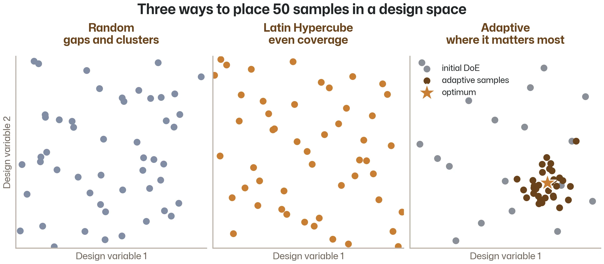
The training data for a surrogate model isn't collected passively — you actively choose which designs to simulate. This choice matters enormously. 200 well-chosen design points will produce a better surrogate than 500 poorly chosen ones.

Random sampling

The simplest approach: generate random designs within your parameter ranges. Easy to implement but inefficient — random samples tend to cluster in some regions and leave gaps in others. You might accidentally oversample the centre of your design space and undersample the edges.

Latin Hypercube Sampling (LHS)

The standard approach for surrogate modelling. LHS ensures that each design variable is sampled evenly across its full range, and the samples are spread across the design space without clustering. Think of it as a multi-dimensional version of stratified sampling.

With 200 LHS points across 6 variables, you get much better coverage than 200 random points. The improvement is especially noticeable in higher dimensions.

Sobol sequences

A quasi-random approach that provides even better space-filling properties than LHS. Sobol sequences are deterministic (reproducible) and fill the design space more uniformly as you add more points. Useful when you might want to add more training points later — new Sobol points naturally fill in the gaps left by previous ones.

Adaptive sampling (Bayesian Optimisation)

The most sophisticated approach: let the surrogate itself decide where to sample next. After training an initial surrogate on a small set of designs, the algorithm identifies regions of the design space where the model is most uncertain or where improvement is most likely, and suggests the next simulation to run.

This is called Bayesian Optimisation when the goal is to find the optimal design. It's remarkably efficient — finding near-optimal designs in 30–50 evaluations that would require thousands with grid search. The GP's uncertainty estimates make this possible: the algorithm can distinguish between "I'm confident this region is bad" and "I haven't explored this region yet."

Optimisation with surrogates: the real payoff

Building a surrogate is valuable on its own — you can explore the design space interactively, understand sensitivities, and generate response surface plots in seconds. But the real power emerges when you use the surrogate for design optimisation.

Single-objective optimisation

"Find the lightest bracket that keeps maximum stress below 250 MPa and first natural frequency above 50 Hz."

Without a surrogate: you'd need an optimisation algorithm that calls the FEA simulation at every iteration. With 200 evaluations and 45 minutes each, that's 150 hours — and the optimiser might need 500+ evaluations to converge.

With a surrogate: the optimiser calls the ML model instead. Each evaluation takes milliseconds. You can run 100,000 evaluations in seconds. The optimiser converges quickly, and you verify the final design with one real simulation to confirm.

Multi-objective optimisation

"Show me the trade-off between weight and maximum stress — the full Pareto front."

This requires evaluating hundreds or thousands of designs across the trade-off surface. Computationally intractable with direct simulation. Trivial with a surrogate.

The result is a Pareto front — a curve showing the best achievable stress for each weight level (or vice versa). The engineer picks their preferred trade-off point, and the surrogate can tell them exactly which design variables achieve it.

Constraint satisfaction

"Which designs satisfy all my constraints simultaneously?"

With a surrogate, you can evaluate the entire design space and colour-code it: green for feasible (all constraints met), red for infeasible. This "feasibility map" gives engineers an intuitive understanding of how large the feasible region is, which constraints are most restrictive, and where the boundaries lie.

A practical example: cantilever beam surrogate

To make this concrete, here's a simplified workflow for building a surrogate of a cantilever beam FEA model:

     
from sklearn.model_selection import cross_val_score
from sklearn.ensemble import GradientBoostingRegressor
from scipy.stats.qmc import LatinHypercube
import numpy as np

# Step 1: Define the design space
# 4 variables: length (100-300mm), width (20-60mm),
#              height (30-80mm), load (500-5000N)
n_variables = 4
n_samples = 200

# Step 2: Generate training designs with Latin Hypercube Sampling
sampler = LatinHypercube(d=n_variables, seed=42)
samples = sampler.random(n=n_samples)

# Scale to physical ranges
lower_bounds = np.array([100, 20, 30, 500])
upper_bounds = np.array([300, 60, 80, 5000])
X = samples * (upper_bounds - lower_bounds) + lower_bounds

# Step 3: Run simulations (in practice, this calls your FEA solver)
# Here we'd use: y = run_fea(X)  for each row
# For demonstration, imagine y contains max stress for each design

# Step 4: Train the surrogate
model = GradientBoostingRegressor(n_estimators=200, max_depth=4,
                                   learning_rate=0.05, random_state=42)

# Step 5: Evaluate with cross-validation
scores = cross_val_score(model, X, y, cv=5, scoring='r2')
print(f"Surrogate R²: {scores.mean():.3f} ± {scores.std():.3f}")

# Step 6: Train on all data and use for predictions
model.fit(X, y)

# Now predict stress for any new design — instantly
new_design = np.array([[200, 40, 50, 2000]])  # length, width, height, load
predicted_stress = model.predict(new_design)
print(f"Predicted max stress: {predicted_stress[0]:.1f} MPa")
                    

The entire workflow uses tools you've already learned in this knowledge base: Latin Hypercube Sampling for DOE, cross-validation for honest evaluation, gradient boosting for the model. The only new element is the context — you're predicting simulation outputs instead of experimental measurements.

When surrogates work well — and when they don't

They work well when:

• The simulation is expensive (minutes to hours per run)
• The design space has a moderate number of variables (3–15)
• The response surface is reasonably smooth
• You need to evaluate many designs (optimisation, sensitivity studies, design space exploration)
• The operating region is well-defined (you know the bounds of your design variables)

They struggle when:

• The response surface has sharp discontinuities (sudden mode changes, buckling)
• The design space is very high-dimensional (50+ variables) — you need exponentially more training points
• You need predictions outside the training range (extrapolation) — surrogates are interpolation tools, not extrapolation tools
• The simulation is cheap enough that you don't need a shortcut (if it runs in 5 seconds, just run it directly)
• Accuracy requirements are extremely tight (±0.1%) — surrogates are approximations, and there's always some error

Why this concept matters for engineers specifically

Surrogate modelling is the article in this knowledge base that no generic ML course covers. Every ML course teaches Random Forest and XGBoost. Very few teach you to replace a 4-hour CFD simulation with a millisecond ML prediction.

This is the concept that makes ML uniquely valuable in engineering contexts — not because it's technically more difficult than defect detection or process optimisation, but because it connects ML directly to the simulation-driven workflows that define modern engineering. Every engineer who runs FEA, CFD, multi-body dynamics, or electromagnetic simulations can benefit from surrogate modelling. And now you understand the concept well enough to try it.

Key takeaways

A surrogate model replaces an expensive simulation with a fast ML approximation. Train on a few hundred simulation results, predict for millions of new designs in seconds.

The workflow is: DOE → simulate → train → evaluate → optimise. Latin Hypercube Sampling for efficient coverage, cross-validation for honest evaluation, and any regression algorithm for the model itself.

Gaussian Processes are ideal for surrogates because they provide uncertainty estimates and produce smooth predictions. XGBoost and polynomial regression are strong alternatives depending on the problem.

Design of Experiments matters as much as the algorithm. Well-chosen training points (LHS, Sobol, adaptive sampling) dramatically outperform random sampling. 200 good points beat 500 bad ones.

The real payoff is optimisation. Once you have a fast surrogate, you can explore the full design space, map Pareto fronts, and find optimal designs in seconds rather than weeks.

This is ML's unique value proposition for engineers. No other application of ML is as directly connected to the simulation-driven workflows that define modern engineering practice.