k-Nearest Neighbours

The algorithm that needs no training

Every other algorithm in this knowledge base learns something during training — weights, split points, tree structures. The model is built once, then applied to new data.

k-Nearest Neighbours (k-NN) doesn't learn anything. There's no training step. There's no model to save. The algorithm simply stores the entire training dataset and uses it directly at prediction time.

When you ask it to predict for a new data point, it does exactly what you'd do intuitively:

For regression, it averages the labels of those k neighbours. For classification, it takes a majority vote.

That's the entire algorithm. No cost function, no gradient descent, no trees, no weights. Just "find the closest examples and do what they did."

An engineering analogy you've already used

You do k-NN every day without realising it.

When a new manufacturing problem comes up — say, a batch of parts is showing unexpected warpage — what does an experienced engineer do? They think: "Have we seen conditions like this before? What happened last time?" They mentally search through past cases, find the ones most similar to the current situation, and use those past outcomes to predict what's going on now.

That's k-NN. The algorithm just does it systematically, across more variables and more historical data than a person can hold in their head.

An injection moulding engineer might think: "The last three times we ran with melt temperature around 215°C, injection pressure around 78 bar, and cooling time around 14 seconds, the shrinkage was 1.8%, 2.0%, and 1.9%. So for this new run with similar settings, I'd expect about 1.9%."

That engineer just performed 3-nearest-neighbours regression in their head.

How "similar" is defined: distance metrics

The core question in k-NN is: how do you measure which data points are "closest" to the new one?

The most common approach is Euclidean distance — the straight-line distance between two points, extended to as many dimensions as you have features. For two data points with features (temperature, pressure, speed), the distance is calculated the same way you'd calculate the distance between two points in 3D space.

This works well when all features are on similar scales. But here's a critical pitfall: if your features have very different scales, the distance calculation is dominated by the feature with the largest values.

Consider two CNC machining parameters:

• Spindle speed: ranges from 800 to 3,000 rpm
• Depth of cut: ranges from 0.5 to 3.0 mm

Without scaling, a difference of 100 rpm (trivial in practice) would count far more than a difference of 1 mm in depth of cut (significant in practice), simply because the rpm numbers are larger.

The fix: always scale your features before using k-NN. Standardisation (subtract the mean, divide by the standard deviation) puts all features on the same scale so no single feature dominates the distance calculation.

     
from sklearn.preprocessing import StandardScaler

scaler = StandardScaler()
X_train_scaled = scaler.fit_transform(X_train)
X_test_scaled = scaler.transform(X_test)  # use the same scaling as training
                    

Choosing k: how many neighbours?

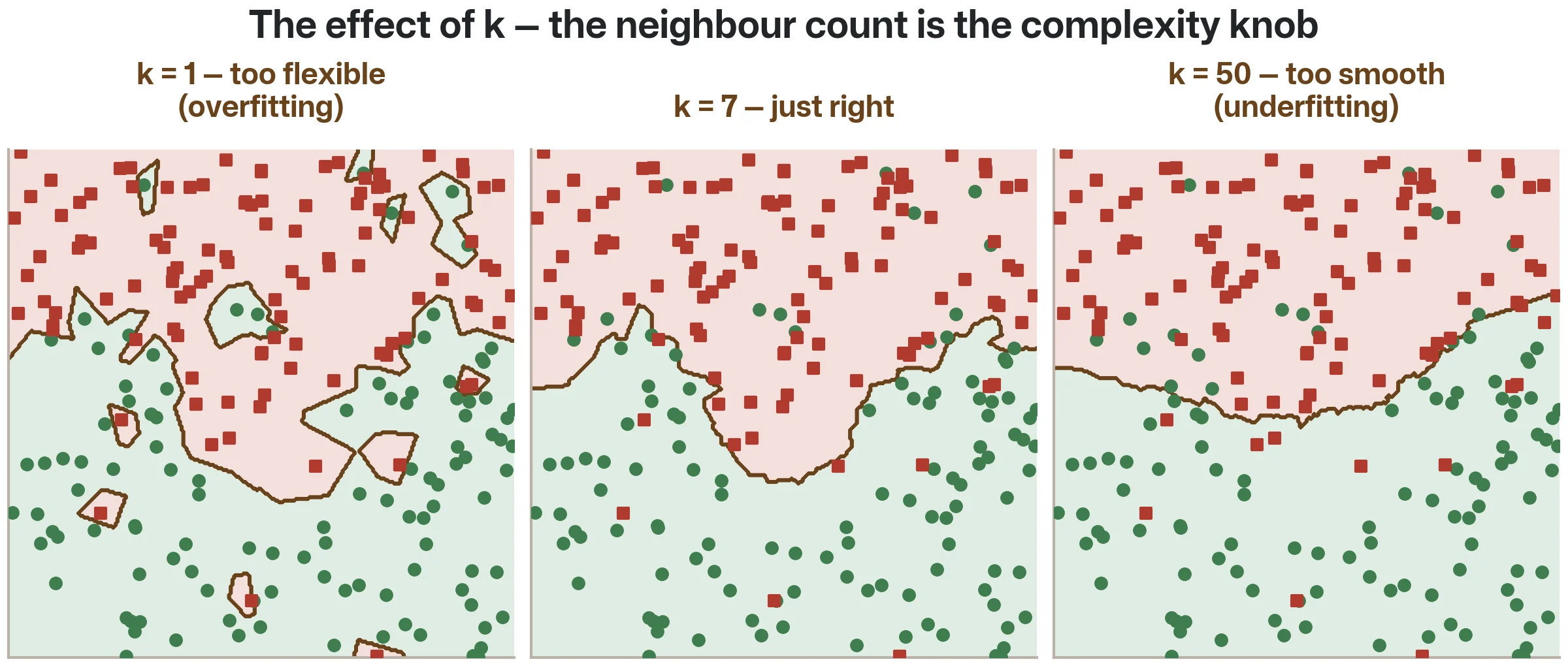
The number of neighbours k is the algorithm's only real hyperparameter, and it directly controls the bias-variance trade-off you learned about in the Overfitting and Underfitting article.

k = 1 (one nearest neighbour): the prediction is entirely determined by the single closest training point. This is the most flexible setting — the model can capture very local patterns. But it's also the most sensitive to noise. One mislabelled or unusual training point will produce a wrong prediction for any new point that happens to be nearby. This is overfitting.

k = 100 (many neighbours): the prediction is averaged over 100 training points. This is very smooth and stable — individual noisy points have little influence. But it might also smooth away real local patterns, making all predictions look like the global average. This is underfitting.

The sweet spot is usually somewhere in between. Common starting values are k = 5 for small datasets and k = 10–20 for larger ones. The best approach is to try several values and compare test set performance — or use cross-validation (covered in Stage 3).

A useful rule of thumb: k should be odd for binary classification (to avoid ties in the majority vote). For regression, ties aren't an issue since you're averaging numbers.

When k-NN works well

Small datasets with low-to-moderate dimensionality. With a few hundred samples and 5–15 features, k-NN can be surprisingly effective. It doesn't make any assumptions about the shape of the relationship — it's purely data-driven. If the true pattern is weird, non-linear, and impossible to describe with an equation, k-NN doesn't care. It just looks at what happened nearby.

Interpolation problems. If you're predicting within the range of your training data (not extrapolating beyond it), k-NN is a natural fit. It literally says "your new data point is similar to these known points, so the answer is probably similar too." This is the ML equivalent of reading values off a graph between known data points.

Quick baselines. k-NN requires almost no decisions — choose k, scale the features, done. It's the fastest way to get a first estimate of whether ML can solve your problem at all. If k-NN gives decent results, you know there are patterns in the data worth finding with more sophisticated methods.

Material property estimation. Given a new alloy composition, find the 5 most similar compositions in your test database and average their measured properties. This is a natural application because engineers intuitively think about material similarity — k-NN formalises that intuition.

When k-NN falls short

High-dimensional data. As the number of features grows, something counterintuitive happens: all data points become approximately equally distant from each other. In a 50-dimensional space, the concept of "nearest neighbour" becomes meaningless because the distances all converge. This is known as the curse of dimensionality, and it's the primary limitation of k-NN.

For engineering datasets with more than 15–20 features, k-NN usually performs poorly unless you first reduce the dimensionality (using PCA or feature selection).

Large datasets. Because k-NN stores the entire training set and searches through it at every prediction, prediction time grows linearly with the number of training samples. With 10,000 samples, each prediction requires calculating 10,000 distances. This is manageable. With 1,000,000 samples, it's slow. Tree-based models, by contrast, make predictions in milliseconds regardless of training set size.

Extrapolation. k-NN cannot extrapolate beyond the range of the training data. If all your training data has temperatures between 150°C and 250°C, and you ask for a prediction at 300°C, k-NN will simply return the average of the nearest points — which are all near 250°C. It has no way to project the trend beyond what it's seen. Linear regression and tree-based models share this limitation to some degree, but k-NN is the most obviously affected.

Noisy data with many irrelevant features. Every feature contributes equally to the distance calculation (after scaling). If half your features are noise, they'll push the distance calculation in random directions, making the "nearest" neighbours not actually similar in any meaningful way. Tree-based models handle irrelevant features naturally (they just don't split on them). k-NN has no such mechanism.

k-NN in Python

Here's the complete workflow, following the same pattern you've seen throughout this knowledge base:

     
from sklearn.neighbors import KNeighborsRegressor
from sklearn.preprocessing import StandardScaler
from sklearn.model_selection import train_test_split
from sklearn.metrics import mean_squared_error
import numpy as np

# Assume X = features, y = labels
# Example: predicting thermal conductivity from composite material properties
X_train, X_test, y_train, y_test = train_test_split(X, y, test_size=0.2, random_state=42)

# CRITICAL: Scale features before k-NN
scaler = StandardScaler()
X_train_scaled = scaler.fit_transform(X_train)
X_test_scaled = scaler.transform(X_test)

# Train a k-NN model
model = KNeighborsRegressor(n_neighbors=5)
model.fit(X_train_scaled, y_train)

# Evaluate
predictions = model.predict(X_test_scaled)
rmse = np.sqrt(mean_squared_error(y_test, predictions))
print(f"RMSE: {rmse:.3f}")
                    

Two things to notice:

The scaling step is new. This is the first algorithm in this knowledge base that requires feature scaling. Random Forest and XGBoost don't need it — but k-NN absolutely does. If you forget this step, your model will be dominated by whichever feature has the largest numeric range.

There are no feature importances. Unlike tree-based models, k-NN doesn't tell you which features matter. It treats all features equally (after scaling). If you need to know which inputs drive the prediction, use a tree-based model or add SHAP analysis (Stage 4).

Where k-NN fits in your toolkit

At this point in the knowledge base, you've met five algorithms:

Algorithm	Strengths	Best for
Linear Regression	Interpretable, fast, works with small data	Linear relationships, baselines, feature importance
Decision Tree	Fully transparent, handles non-linearity	Interpretability, teaching overfitting
Random Forest	Robust, minimal tuning, stable	First serious model, reliable performance
XGBoost	Highest accuracy on tabular data	Maximum performance, after tuning
k-NN	Simple, no assumptions, good for interpolation	Small datasets, quick baselines, material lookup

Each has a role. Linear regression is your first check ("is there a simple relationship here?"). k-NN is your second check ("is there any pattern, regardless of shape?"). Random Forest is your reliable workhorse. XGBoost is your performance maximiser.

In practice, most engineering ML projects end up using Random Forest or XGBoost for the final model. But k-NN and linear regression often appear in the exploration phase — quick experiments that tell you whether the problem is solvable before you invest time in tuning a more powerful model.

This completes Stage 2. You now know the core algorithms used in the vast majority of engineering ML work. Stage 3 will teach you to evaluate these models honestly — because a model is only as useful as your ability to measure how good it actually is.

Key takeaways

k-NN predicts by finding similar past examples. No training, no model — just "find the k closest data points and use their values." It formalises the engineering instinct of reasoning from precedent.

Always scale your features. Unlike tree-based models, k-NN uses distances between data points. If features have different scales, the largest-scale feature dominates. Standardise everything first.

k controls the bias-variance trade-off. Low k = flexible but noisy (overfitting risk). High k = smooth but may miss local patterns (underfitting risk). Try several values and compare test performance.

k-NN struggles with many features. The curse of dimensionality makes "nearest neighbour" meaningless in high-dimensional space. Keep the feature count moderate, or reduce dimensions first.

Use k-NN for quick baselines and small-data interpolation. It's rarely the best final model, but it's invaluable for early exploration: if k-NN works, there are patterns worth finding. If k-NN fails, more complex models may struggle too.